Quickstart

This walk-through takes you from a stock Kale install to a running pipeline on Kubeflow Pipelines in under ten minutes, using the candies_sharing example that ships with the repository.

The recommended path is the JupyterLab UI: you annotate cells, compile, and submit the pipeline without ever leaving the notebook. If you’d rather drive Kale from a terminal, the CLI flow at the bottom of this page covers the same journey.

Prerequisites

Before you start, make sure you have:

• Kale installed, including the JupyterLab extension (see Installation).

• A running Kubernetes cluster with Kubeflow Pipelines v2.16.0+ deployed.

• The KFP API reachable on http://127.0.0.1:8080 — for a minikube setup you can run:

  kubectl port-forward -n kubeflow svc/ml-pipeline-ui 8080:80
  

1. Launch JupyterLab with Kale

From the repository root, start the bundled JupyterLab environment:

make jupyter

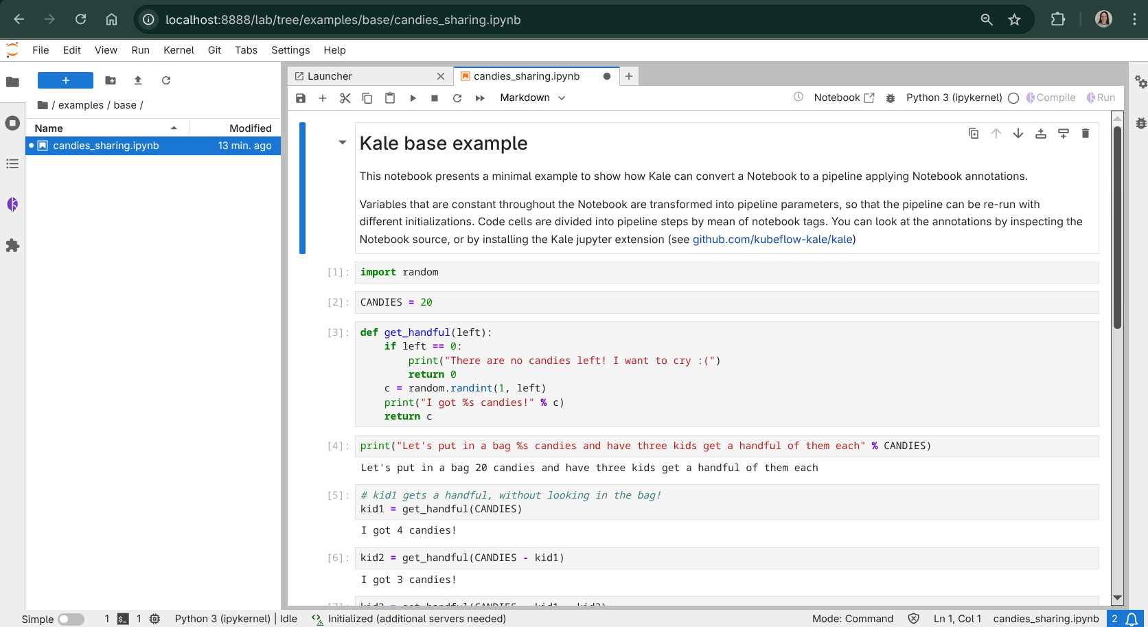
Then open examples/base/candies_sharing.ipynb from the file browser. The notebook defines a toy pipeline that demonstrates every Kale concept in the minimum amount of code, and it ships already annotated with Kale tags.

2. Open the Kale side panel

Click the Kale icon in the JupyterLab left sidebar to toggle the Kale Deployment Panel. This is the control surface you’ll use for the rest of the quickstart: it inspects cell tags, compiles the notebook, and submits runs to Kubeflow Pipelines.

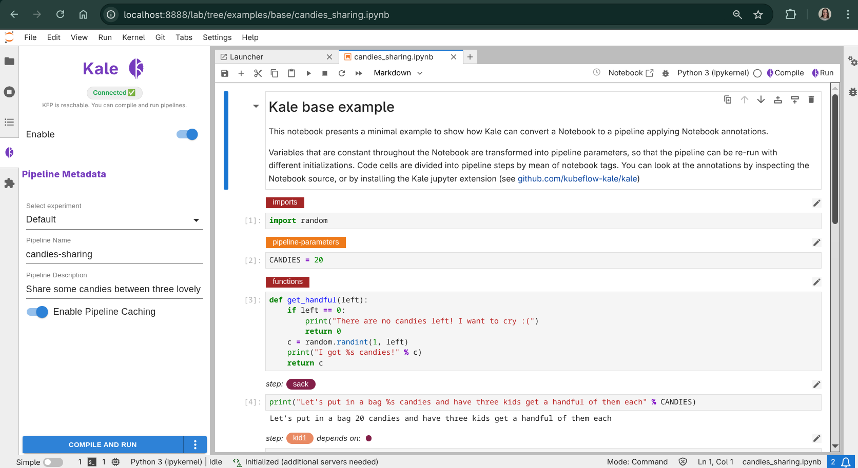
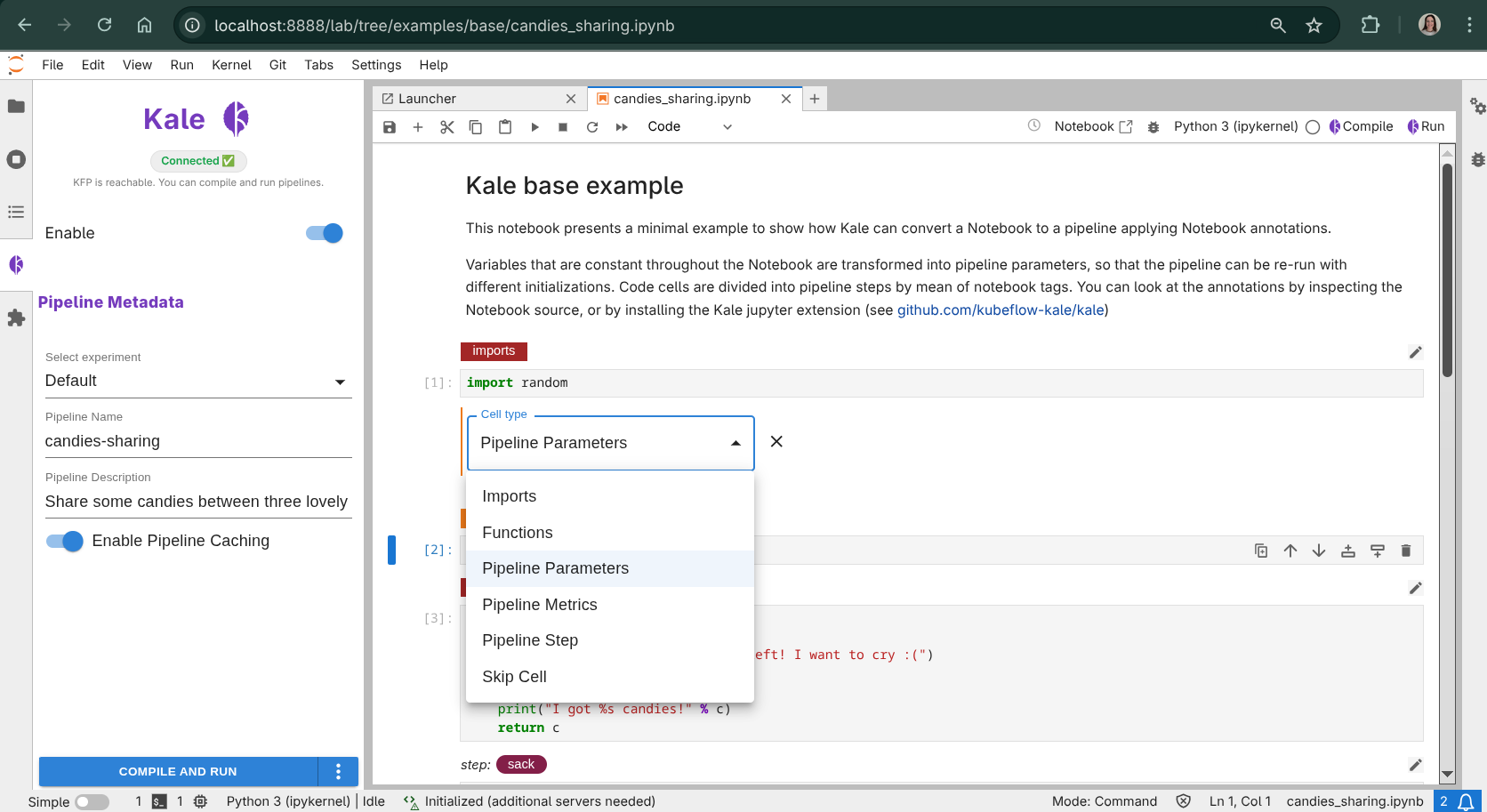
3. Review the cell tags

Each cell now has a dropdown showing its Kale cell type. The candies_sharing notebook uses most of Kale’s core tag types:

• Imports — all import statements go here. Kale prepends this cell to every step in the pipeline.

• Pipeline Parameters — defines values that will become KFP parameters, tweakable at submission time.

• Step — one or more named steps, each with optional dependencies on earlier steps (declared via prev:<step_name>).

See Cell Types & Annotations for the full tag vocabulary.

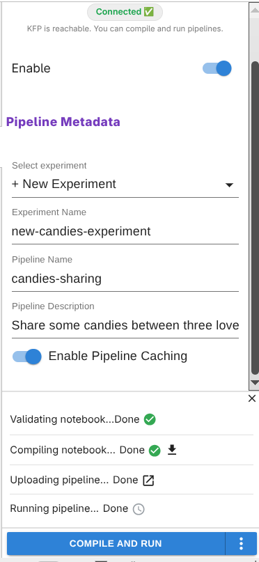
4. Configure the pipeline metadata

In the Kale side panel, confirm the basics:

• Pipeline name — defaults to the notebook filename.

• Experiment — defaults to Default (or the first available KFP experiment).

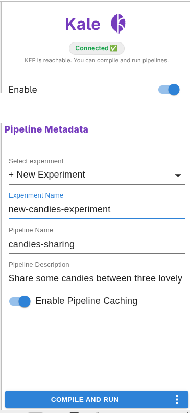
5. Compile and run from the panel

Click Compile and Run at the bottom of the Kale panel. Kale will, in order:

1. Parse the notebook and extract the Kale tags from cell metadata.

2. Build a pipeline DAG (Directed Acyclic Graph) from the step and prev: annotations.

3. Detect which variables need to flow between steps.

4. Generate a KFP v2 DSL Python script under .kale/.

5. Upload the pipeline to KFP and start a new run in the selected experiment.

Each phase updates in place in the panel, with a link to the generated .kale/<notebook>.kale.py once it exists.

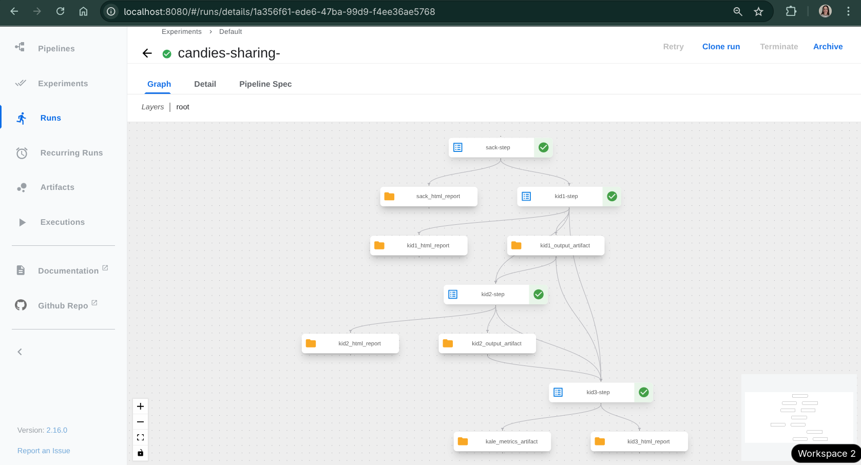
6. Watch the run in the KFP UI

When the upload finishes, the panel shows a View run link pointing at the Kubeflow Pipelines UI. Follow it to watch the DAG execute step-by-step; click any step to see its logs, artifacts, and the data Kale marshalled in and out of it.

What’s next?

• Learn how Kale detects and moves data between steps in Data Passing & Marshalling.

• Explore the rest of the panel (volumes, snapshots, parameters) in Running Pipelines.

• Browse the examples gallery for more realistic pipelines.

---

Advanced: CLI flow

If you’d rather drive Kale from a terminal — for example in CI, on a remote box without a JupyterLab install, or when scripting multi-notebook builds — you can do the same thing with the kale CLI.

Compile the notebook

kale --nb examples/base/candies_sharing.ipynb

Look inside the .kale/ directory that was just created:

ls .kale/
# candies_sharing.kale.py     ← generated KFP v2 DSL

Open candies_sharing.kale.py — you’ll see one @kfp_dsl.component function per step, a @kfp_dsl.pipeline function wiring them together, and a __main__ block that you can run directly to compile the pipeline to YAML.

Compile and submit in one step

Add --run_pipeline to compile and submit the pipeline to KFP in one shot:

kale --nb examples/base/candies_sharing.ipynb \
     --kfp_host http://127.0.0.1:8080 \
     --run_pipeline

This uploads the pipeline, creates an experiment (default: Kale-Pipeline-Experiment), and starts a run. Open the KFP UI at http://127.0.0.1:8080 and navigate to Runs to watch it execute.

See CLI Reference for the complete CLI reference.